resources for biostatistics
resources for biostatistics
Table of Contents
-
1. Lesson 8 — 3D scatterplot
Learning Objectives
Create 3D scatterplots
Demonstration
Here is the dataset that we are using in this demo:
This dataset is about Down’s Syndrome in Canada. (I have slightly modified the original dataset for our purpose).
https://vincentarelbundock.github.io/Rdatasets/doc/boot/downs.bc.html
We will first import the dataset. Then we will generate a 3D scatterplot from the dataset downs_bc. See below for details.
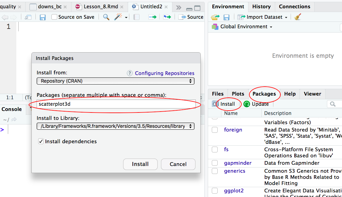
Step 1: Install the R package “scatterplot3d”
Two ways to install a R package one way is to type install.packages(scatterplot3d); the other way is to install via the graphical interface of RStudio:
Step 2: Install the R package “scatterplot3d”
Before we can use the R package to create 3D scatterplots, we need to load the package into R first:
> library(scatterplot3d)
Step 3: Create a 3D scatterplot
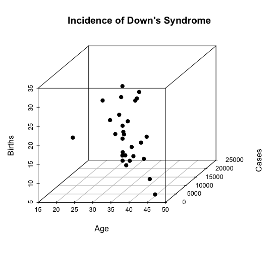
Our dataset is called downs_bc. We want to generate a 3D scatterplot for the three columns in that dataset: cases, age and births.
> library(scatterplot3d)
> with(downs_bc,
+      scatterplot3d(cases ~ age + births, pch = 19,
+                    main="Incidence of Down's Syndrome",
+                    xlab="Age", ylab="Cases", zlab="Births"))
Explanation:
We use the library function to load the R package “scatterplot3d“.
Then we use generate the 3D scatterplot from the databset downs_bc:
cases ~ age means that the variable cases is explained by age (i.e. age is the explanatory variable);
+ births means that the variable births is the third variable in this scatterplot;
pch = 19 means to use plotting symbol 19 (solid circle) in our plot. (Type ?pch at the prompt to find out more about pch.)
Here is the 3D scatterplot:
-END-
-
2. Lesson 9—Import data via R scripts
Learning Objectives
Write code to important data in .R scripts
Demonstration
Instead of using the Import Dataset button in RStudio as we have been doing so far, we will write R codes in our .R script to do the data importing.
The advantage of importing your data via your .R script is that you can re-import your dataset and re-run your script in one smooth operation so as to generate a clean output.
Here are the steps:
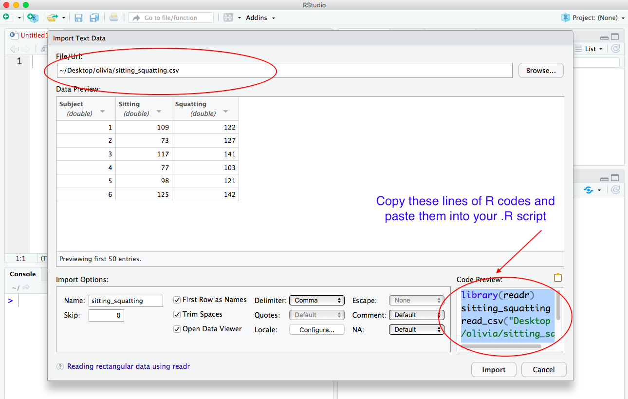
Step 1: Bring up the Import Dataset screen
In RStudio,
i) Click the Import Dataset button and choose From Text (readr)….
ii) Then select the dataset that you are going to use BUT DO NOT click the IMPORT button at the bottom of the screen yet.
iii) Instead, copy the lines of R code in the box Code Preview in the lower left-hand corner of the screen and then paste the lines of R code into your .R script.
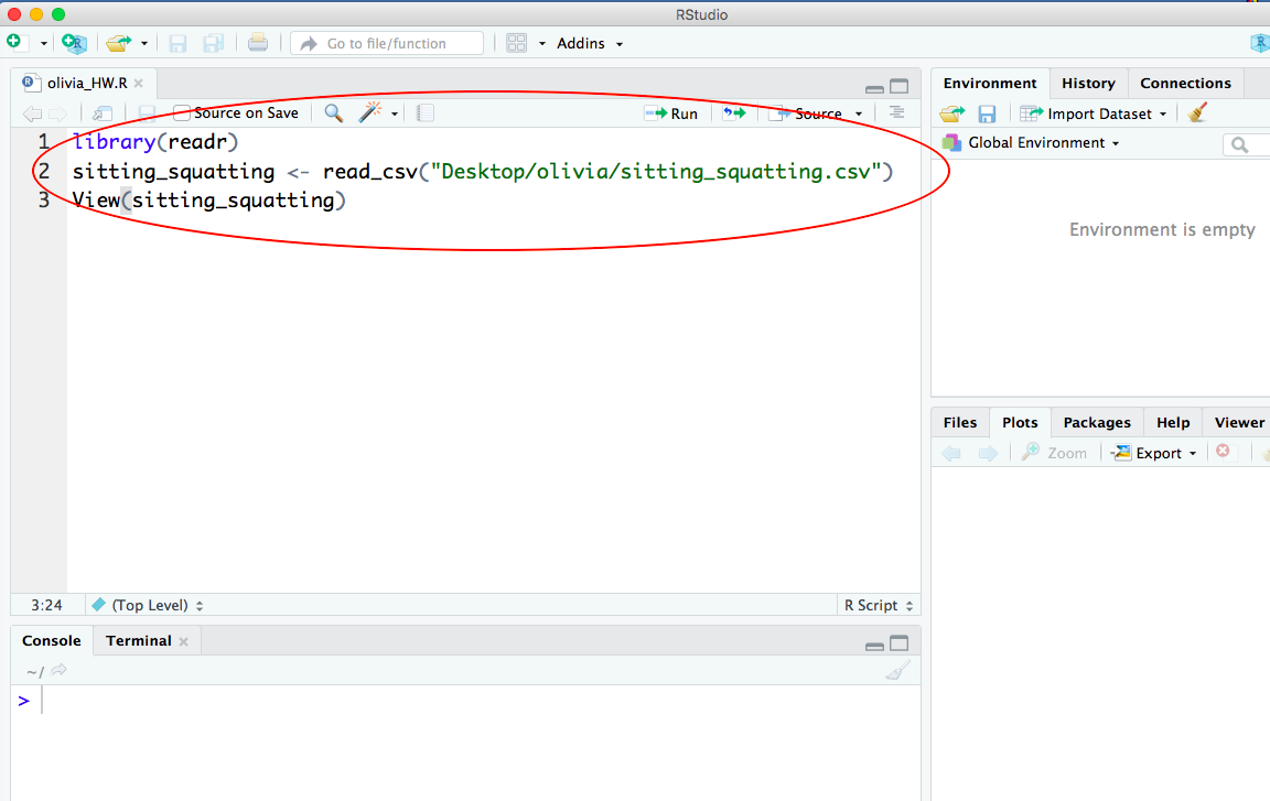
Here is what your .R script should look like after you paste the lines of R code and save your script:
-END-
-
3. Lesson 10—Matched-Pairs t tests
Learning Objectives
Perform a matched-pair hypothesis t test
Demonstration
Here is the dataset that we are using in this demo from #17.16 in our textbook:
Goal: To conduct a two-sided t test of no difference for a matched-pair t test
Here are the null and alternative hypotheses in this example:
\(H_0: \mu_1 = \mu_2 \)
\(H_a: \mu_1 \neq \mu_2 \)
where
\( \mu_1 \) = population mean angle in squatting
\( \mu_2 \)= population mean angle in sitting
Here are the steps:
Step 1: Import the dataset
Step 2: Create a column of difference
w = sitting_squatting$Sitting - sitting_squatting$Squatting
DO NOT use name your column of difference as diff because diff is a built-in function in R.
In this demonstration, we name our column of difference w.
Step 3: Draw a stemplot to check data
Draw a stemplot on the column of difference to check if data are roughly symmetric and without too many extreme outliers:
stem(w)
Step 3: Run the matched-pair t test via the R function t.test
t.test(sitting_squatting$Sitting, sitting_squatting$Squatting,
               mu=0, paired=TRUE,
               conf.level = 0.95)
Explanation:
Whenever R runs a hypothesis test, R automatically calculates the corresponding confidence interval —the range of values which the population mean is estimated to lie within.
Given a set of data, the corresponding hypothesis test result and the confidence interval are closely related. Therefore if we want the significance level \(\alpha \) to be 0.05, then we set the argument conf.level = 0.95 because conf.level = 1 – \(\alpha \) .
By default, R automatically sets \(\mu = 0 \) and conf.level = 0.95 even if you don’t explicitly type these arguments. So you can skip typing these arguments into the t.test function if you are testing a two-sided alternative hypothesis with \(\alpha =0.05\).
-END-
-
4. Lesson 11—Two-Sample t tests
Learning Objectives
Perform a two-sample t hypothesis test
Demonstration
Goal:
To conduct a two-sample t test with a two-sided alternative hypothesis. The following example to test if there is a difference between heights of plants grown with and without fertilizers (see p111 in [1]).
Here are the null and alternative hypotheses in this example:
\(H_0: \mu_1 = \mu_2 \)
\(H_a: \mu_1 \neq \mu_2 \)
where
\( \mu_1 \) = population mean height of plants grown without fertilizers
\( \mu_2 \)= population mean height of plants grown with fertilizers
Here are the steps:
Step 1: Enter the data
We create a vector called cont to store heights of plants grown without fertilizers.
cont = c(64.7, 86.6, 67.1, 62.6, 75.1, 83.8, 71.7, 83.4, 90.3, 82.7)
We then create another vector called fert to store heights of plants grown with fertilizers.
fert = c(110.3, 130.4, 114.0, 135.7, 129.9, 98.2, 109.4, 131.4, 127.9, 125.7)
Step 3: Draw boxplots to check data
We draw two boxplots to check if the data are roughly symmetric and without too many extreme outliers:
boxplot(cont, fert, names =c("Control", "Fertilizer"),
        xlab = "Treatment", ylab = "Plant Height (cm)",
        main = "Plants with(out) Fertilizer", cex.lab =1.5)
Explanation:
The argument cex.lab magnifies the labels (default value is 1).
Step 4: Run the two-sample t test via the R function t.test
t.test(cont, fert, mu = 0, conf.level = 0.99)
Explanation:
Whenever R runs a hypothesis test, R automatically calculates the corresponding confidence interval —the range of values which the population mean is estimated to lie within.
Given a set of data, the corresponding hypothesis test result and the confidence interval are closely related. Therefore if we want the significance level \(\alpha \) to be 0.01, then we set the argument conf.level = 0.99 because conf.level = 1 – \(\alpha \) .
By default, R automatically sets mu=0 and conf.level = 0.95 even if you don’t explicitly type these arguments. So you can skip typing these arguments into the t.test function if you are testing a two-sided alternative hypothesis with \(\alpha =0.05\).
References
[1] Hartvigsen, G. 2014. A Premier in Biological Data Analysis and Visualization Using R. Columbia University Press.
-END-
-
5. Lesson 12—The Chi-Square Test for Goodness of Fit
Learning Objectives
Perform a chi-square goodness-of-fit test.
Demonstration
Goal: To conduct a chi-square goodness-of-test for #21.24 in our textbook.
For #21.24, the null hypothesis is:
\(H_0: p_{tall} = 0.75, p_{dwarf} = 0.25 \)
Here is the R code:
chisq.test(c(787, 277), p=c(0.75, 0.25))
Explanation:
We use the R function chisq.test to run a chi-square test.
The arguments for the chisq.test function are:
c(787, 277) is the vector that stores the two observed values
p=c(0.75, 0.25) is the vector that stores the probabilities in the theoretical model (ratio 3:1). (We must use the letter p but not any other letters in this chisq.test function).
-END-